Deep Dive into ADM Gradient Boosting Models

ADM Gradient Boosting (AGB) models are tree-based models used in Pega as an alternative to the traditional Bayesian approach. While Prediction Studio shows high-level information about predictors and performance, the exported tree structure contains much richer diagnostic data.

This notebook shows how to:

• Load an exported AGB model and inspect its diagnostic metrics (gain distribution, leaf scores, convergence, split types, feature importance)

• Explore per-tree statistics and per-split gains

• Visualise individual trees and trace the scoring path for a given input

• Replicate the model’s propensity score from the tree structure

To export a model, go to the gradient boosting model page in Prediction Studio and use the Actions button in the top right. We also ship a sample model in the data/ folder.

Imports

from pdstools import datasets
from pdstools.adm import ADMTrees

Importing your own model export

To import your own model, simply feed the path to the ADMTrees class. There are no additional parameters.

# ADMTrees("path/to/model_download.json")

For this example we will use the shipped example dataset, which you can simply import with the following line:

Trees = datasets.sample_trees()

Model diagnostic metrics

The .metrics property computes a comprehensive set of diagnostics from the tree structure — covering performance, complexity, gain distribution, leaf scores, split types, learning convergence, and feature importance concentration. The .metric_descriptions() method provides a human-readable description for each metric.

import polars as pl
from pdstools.adm.ADMTrees import ADMTreesModel

descriptions = ADMTreesModel.metric_descriptions()
metrics = Trees.metrics

pl.DataFrame([
    {"Metric": k, "Value": str(v), "Description": descriptions.get(k, "")}
    for k, v in metrics.items()
]).to_pandas().style.hide()

Metric	Value	Description
auc	None	Area Under the ROC Curve — overall model discrimination power.
success_rate	None	Proportion of positive outcomes in the training data.
factory_update_time	None	Timestamp of the last factory (re)build of this model.
response_positive_count	None	Number of positive responses in training data.
response_negative_count	None	Number of negative responses in training data.
number_of_tree_nodes	2232	Total node count across all trees (splits + leaves).
tree_depth_max	10	Maximum depth of any single tree in the ensemble.
tree_depth_avg	7.8	Average depth across all trees.
tree_depth_std	1.92	Standard deviation of tree depths — uniformity of tree complexity.
number_of_trees	50	Total number of boosting rounds (trees) in the model.
number_of_stump_trees	1	Trees with no splits (single root node). Stumps contribute no learned signal.
avg_leaves_per_tree	22.82	Average number of leaf nodes per tree — a proxy for tree complexity.
number_of_splits_on_ih_predictors	292	Total splits on Interaction History (IH.*) predictors.
number_of_splits_on_context_key_predictors	236	Total splits on context-key predictors (py*, Param.*, *.Context.*).
number_of_splits_on_other_predictors	563	Total splits on customer/other predictors.
total_number_of_active_predictors	41	Predictors that appear in at least one split.
total_number_of_predictors	83	All predictors known to the model (active or not).
number_of_active_ih_predictors	29	Active IH predictors (appear in splits).
total_number_of_ih_predictors	0	All IH predictors in the model configuration.
number_of_active_context_key_predictors	3	Active context-key predictors.
number_of_active_symbolic_predictors	7	Active symbolic (categorical) predictors.
total_number_of_symbolic_predictors	45	All symbolic predictors in configuration.
number_of_active_numeric_predictors	26	Active numeric (continuous) predictors.
total_number_of_numeric_predictors	38	All numeric predictors in configuration.
total_gain	10306.476	Sum of all split gains — total information gained by the ensemble.
mean_gain_per_split	9.4816	Average gain per split node (analogous to XGBoost gain importance).
median_gain_per_split	2.0275	Median gain — robust central tendency, less sensitive to outlier splits.
max_gain_per_split	1102.557	Largest single split gain — identifies the most informative split.
gain_std	57.4547	Standard deviation of gains — high values indicate a few dominant splits.
number_of_leaves	1141	Total leaf nodes across all trees.
leaf_score_mean	-0.016645	Average leaf score (log-odds contribution). Near zero means balanced.
leaf_score_std	0.161401	Spread of leaf scores — wider spread means better discrimination.
leaf_score_min	-0.598675	Most negative leaf score.
leaf_score_max	0.537159	Most positive leaf score.
number_of_numeric_splits	750	Splits using '<' (numeric/continuous thresholds).
number_of_symbolic_splits	283	Splits using 'in' or '==' (categorical membership).
symbolic_split_fraction	0.274	Fraction of splits that are symbolic (0–1).
number_of_unique_splits	379	Distinct split conditions across all trees.
number_of_unique_predictors_split_on	41	Number of distinct predictor variables used in splits.
split_reuse_ratio	2.88	Total splits / unique splits — how often the same condition recurs across trees.
avg_symbolic_set_size	9.77	Average number of categories in symbolic 'in { ... }' splits.
mean_abs_score_first_10	0.308436	Mean |root score| of the first 10 trees — initial correction magnitude.
mean_abs_score_last_10	0.021106	Mean |root score| of the last 10 trees — late correction magnitude.
score_decay_ratio	0.0684	Ratio last/first — values < 1 indicate convergence, >> 1 indicates instability.
mean_gain_first_half	17.0763	Average gain in the first half of trees.
mean_gain_last_half	2.2815	Average gain in the second half — lower values suggest convergence.
top_predictor_by_gain	pyName	Predictor with the highest total gain.
top_predictor_gain_share	0.5481	Fraction of total gain from the top predictor (0–1). High = dominance.
predictor_gain_entropy	0.4206	Normalised Shannon entropy of gain distribution (0–1). Low = concentrated.

The detailed predictor name-to-type mapping is available in the predictors attribute.

Trees.predictors

{'Account.DaysSinceOpened': 'numeric',
 'Account.CurrentDateInt': 'numeric',
 'Customer.IsCustomerActive': 'symbolic',
 'Account.YTDPayments': 'numeric',
 'Customer.HealthMatter': 'symbolic',
 'Customer.LastReviewedDate': 'numeric',
 'Account.YTDBrokenPromises': 'numeric',
 'Customer.NetWealth': 'numeric',
 'Customer.MilitaryService': 'symbolic',
 'Account.DelinquencyAmount': 'numeric',
 'Customer.IsPrimary': 'symbolic',
 'Account.Role': 'symbolic',
 'Customer.NextReviewDate': 'symbolic',
 'Account.type': 'numeric',
 'Param.JourneyStage': 'symbolic',
 'Param.DaysinCurrentStage': 'numeric',
 'Account.InArrears': 'symbolic',
 'Account.PaymentNetwork': 'symbolic',
 'Account.AverageYearlyBalance': 'numeric',
 'Customer.AnnualIncome': 'numeric',
 'Account.YTDOverLimit': 'numeric',
 'Account.BonusMet': 'symbolic',
 'Account.CreditLine': 'numeric',
 'Customer.LanguagePreference': 'symbolic',
 'Param.Journey': 'symbolic',
 'Customer.RelationshipLengthDays': 'numeric',
 'Customer.ReviewDate': 'numeric',
 'Account.CurrentValue': 'numeric',
 'Account.Appl': 'symbolic',
 'Account.AccountSubType': 'symbolic',
 'Customer.BalanceTransaction': 'numeric',
 'Account.BehaviorScore': 'numeric',
 'Param.PriorStageInJourney': 'symbolic',
 'Customer.ResidentialStatus': 'symbolic',
 'Account.YTDDisputes': 'numeric',
 'Account.ProductType': 'symbolic',
 'Account.Active': 'symbolic',
 'Account.MarketSegmentID': 'numeric',
 'Account.CreditLineAvailable': 'numeric',
 'Customer.EmailOptIn': 'symbolic',
 'Account.LoanToValueRatio': 'numeric',
 'Account.YTDForeignTxnFee': 'numeric',
 'Customer.NoOfDependents': 'numeric',
 'Account.CollectionStatus': 'symbolic',
 'Account.AccountDescription': 'symbolic',
 'Account.OpenDateTime': 'numeric',
 'Customer.Bankruptcy': 'symbolic',
 'Customer.SMSOptIn': 'symbolic',
 'Customer.Incarceration': 'symbolic',
 'Customer.HasActivePaymentPlan': 'symbolic',
 'Account.OwnershipType': 'symbolic',
 'Customer.Deceased': 'symbolic',
 'Account.AccountType': 'symbolic',
 'Account.YTDInArrears': 'numeric',
 'Customer.Age': 'numeric',
 'Account.CyclesPastDue': 'numeric',
 'Account.RateType': 'symbolic',
 'Param.LastJourneyStage': 'symbolic',
 'Account.MaturityDate': 'numeric',
 'Account.NumDaysPastDue': 'numeric',
 'Customer.PushNotificationOptIn': 'symbolic',
 'Customer.NaturalDisaster': 'symbolic',
 'Account.AccountBalance': 'numeric',
 'Account.RewardType': 'symbolic',
 'Account.Rate': 'numeric',
 'Customer.pyCountryCode': 'symbolic',
 'Account.TotalDisputes': 'numeric',
 'Account.BrokenPromiseCount': 'numeric',
 'Customer.InHardship': 'symbolic',
 'Account.BonusWindowOpen': 'symbolic',
 'Account.YTDLatePayment': 'numeric',
 'Account.Status': 'symbolic',
 'Account.YTDInterestPaid': 'numeric',
 'Customer.DownloadedMobileApp': 'symbolic',
 'Account.UnpaidPrincipal': 'numeric',
 'Customer.InArrears': 'symbolic',
 'Account.InCollections': 'symbolic',
 'Account.AvgMonthlyBalance': 'numeric',
 'pyDirection': 'symbolic',
 'pyName': 'symbolic',
 'pyChannel': 'symbolic',
 'pyIssue': 'symbolic',
 'pyGroup': 'symbolic'}

Naturally, the raw trees are stored here too. They are stored in the ‘model’ attribute, in a list with each tree in json format. Let’s look at a single tree.

Trees.model[18]

{'score': -0.04167241398182543,
 'gain': 4.903114150998753,
 'split': 'IH.MISSING.MISSING.Churned.pyHistoricalOutcomeCount < 1.0',
 'left': {'score': 0.0015912192864844406,
  'gain': 4.921074965276381,
  'split': 'IH.SMS.Outbound.Accept.pxLastGroupID is Missing',
  'left': {'score': 0.08708304261596726, 'gain': 0.0},
  'right': {'score': -0.19378256055857698, 'gain': 0.0}},
 'right': {'score': -0.07898210064649579,
  'gain': 2.609510949104644,
  'split': 'IH.SMS.Outbound.Accept.pyHistoricalOutcomeCount < 1.0',
  'left': {'score': -0.050025939043392705,
   'gain': 5.284463037230109,
   'split': 'pyName in { PremierChecking }',
   'left': {'score': 0.3483628622864736, 'gain': 0.0},
   'right': {'score': -0.08596541739325182, 'gain': 0.0}},
  'right': {'score': 0.22697292002283817, 'gain': 0.0}}}

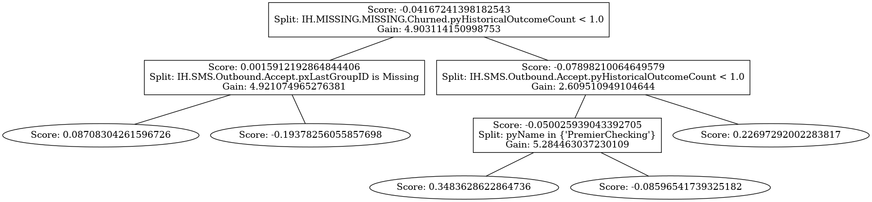
Each node has a ‘score’: the contribution to the final score, over all trees. Non-leaf nodes naturally have splits, which are expressed as a string. These can be inequality, equality or set splits. For example, we may see a split on Age being smaller than 42, but also pyName being one of {P1, P2, P3, P4, P6}. If this split evaluates to True, we follow the tree to the left node. Naturally, if it evaluates to False we follow to the right node. Lastly, each split also has a gain. This describes how well that split discriminates by splitting to the left and right nodes.

Later we will revisit this tree structure, because for visualisation we need to slightly reformat it. But first, by nature of a boosting algorithm, looking at a single tree does not provide enough information to fully understand the model. For this, there are some properties of the ADMTrees class to look across trees. To start, we can call TreeStats to get an overview of the contribution of each tree to the final model.

Trees.tree_stats.sample(5)

shape: (5, 6)

treeID	score	depth	nsplits	gains	meangains
i64	f64	i64	i64	list[f64]	f64
5	-0.26764	6	22	[628.491615, 15.895368, … 4.212203]	32.762797
12	-0.110937	9	30	[142.589623, 20.764557, … 14.075774]	8.546743
19	-0.035604	6	10	[3.549506, 0.113238, … 2.260551]	1.62232
6	-0.243922	7	15	[533.509277, 3.875638, … 2.827234]	39.238225
8	-0.192954	9	38	[443.862522, 9.336564, … 3.842098]	14.86039

In TreeStats, the index is the ‘ID’ of the tree, based on its position in the order of the ‘model’ attribute. The score corresponds to the score of the top-level node of that tree, and the ‘depth’ and ‘nsplits’ describe how deep the tree is, and how many splits are performed in total. For each split, the gain is added to the list in the ‘gains’ column. The mean of all splits in a tree is computed in the ‘meangains’ column.

Some info about individual trees is also stored in attributes, such as the splits and gains for each tree.

print(Trees.splits_per_tree[18])
print(Trees.gains_per_tree[18])

['IH.MISSING.MISSING.Churned.pyHistoricalOutcomeCount < 1.0', 'IH.SMS.Outbound.Accept.pxLastGroupID is Missing', 'IH.SMS.Outbound.Accept.pyHistoricalOutcomeCount < 1.0', 'pyName in { PremierChecking }']
[4.903114150998753, 4.921074965276381, 2.609510949104644, 5.284463037230109]

Variables

Now, if we are interested in the contribution and distribution of the splits per variable, we can look at the raw data in the groupedGainsPerSplit attribute, which returns a DataFrame, grouped by the split. In the ‘gains’ column you see a list of all of the gains produced by this split, and the ‘n’ column says how often this split is performed.

Trees.grouped_gains_per_split

shape: (379, 7)

split	predictor	gains	mean	sign	values	n
str	str	list[f64]	f64	str	object	u32
"pyName in { AutoUsed48Months, …	"pyName"	[177.064524, 95.262737, … 6.283781]	58.111616	"in"	{'IdentityTheftProtection', 'PaymentProtection', 'FirstMortgageSevenOneARM', 'PremiumBanking', 'AMEXPersonal', 'CompleteYourCardApplicationToday', 'GetAPersonalizedRateQuoteToday', 'PlatinumRewardsCard', 'AutoUsed84Months', 'IncreaseYourCreditLine', 'FirstMortgageFloat', 'FirstMortgage', 'StudentChoice', 'ProsAndConsOfFixedRate', 'UFixedRateMortgage', 'AutoNew60Months', 'UPlusProductBundles', 'AutoUsed48Months', 'FirstMortgage30yr', 'SuperSaver', 'MasterCardGold', 'IndividualRetirementAccountsIRA', 'AutoNew84Months', 'Earn2xRewardsPoints', 'HomeOwners', 'CreditMonitoringService', 'PremierChecking', 'AutoUsed36Months', 'UPlusGold', 'MasterCardWorld', 'BasicChecking', 'SignupForRewardsCard', 'VisaGold', 'MoneyMarketSavingsAccount', 'FirstMortgageFiveOneARM'}	5
"pyName in { AutoUsed48Months, …	"pyName"	[1102.556954, 153.075758, … 2.770062]	144.75059	"in"	{'IdentityTheftProtection', 'PaymentProtection', 'FirstMortgageSevenOneARM', 'PremiumBanking', 'AMEXPersonal', 'CompleteYourCardApplicationToday', 'GetAPersonalizedRateQuoteToday', 'PlatinumRewardsCard', 'AutoUsed84Months', 'IncreaseYourCreditLine', 'FirstMortgageFloat', 'FirstMortgage', 'StudentChoice', 'ProsAndConsOfFixedRate', 'UFixedRateMortgage', 'AutoNew60Months', 'UPlusProductBundles', 'AutoUsed48Months', 'FirstMortgage30yr', 'SuperSaver', 'MasterCardGold', 'IndividualRetirementAccountsIRA', 'AutoNew84Months', 'Earn2xRewardsPoints', 'HomeOwners', 'CreditMonitoringService', 'AutoUsed36Months', 'UPlusGold', 'MasterCardWorld', 'SignupForRewardsCard', 'VisaGold', 'FirstMortgageFiveOneARM'}	14
"pyName in { UPlusGold }"	"pyName"	[3.648124, 5.092834, … 1.945262]	3.336998	"in"	{'UPlusGold'}	9
"pyName in { AutoUsed48Months, …	"pyName"	[1.687369, 3.857415, … 2.235231]	1.985773	"in"	{'FirstMortgageSevenOneARM', 'PremiumBanking', 'AMEXPersonal', 'CompleteYourCardApplicationToday', 'PlatinumRewardsCard', 'AutoUsed84Months', 'IncreaseYourCreditLine', 'FirstMortgageFloat', 'FirstMortgage', 'StudentChoice', 'AutoNew60Months', 'UPlusProductBundles', 'AutoUsed48Months', 'FirstMortgage30yr', 'SuperSaver', 'MasterCardGold', 'AutoNew84Months', 'Earn2xRewardsPoints', 'HomeOwners', 'AutoUsed36Months', 'UPlusGold', 'MasterCardWorld', 'VisaGold', 'FirstMortgageFiveOneARM'}	8
"IH.Web.Inbound.Rejected.pxLast…	"IH.Web.Inbound.Rejected.pxLast…	[5.216521, 9.372519, 4.885585]	6.491542	"<"	{'0.9332044675925926'}	3
…	…	…	…	…	…	…
"Customer.NetWealth < 19845.0"	"Customer.NetWealth"	[1.250128]	1.250128	"<"	{'19845.0'}	1
"Customer.NetWealth < 7557.0"	"Customer.NetWealth"	[0.180002]	0.180002	"<"	{'7557.0'}	1
"Customer.RelationshipLengthDay…	"Customer.RelationshipLengthDay…	[2.206005]	2.206005	"<"	{'1122.0'}	1
"Customer.NetWealth < 18233.0"	"Customer.NetWealth"	[0.460809]	0.460809	"<"	{'18233.0'}	1
"IH.Web.Inbound.Accepted.pxLast…	"IH.Web.Inbound.Accepted.pxLast…	[1.215137]	1.215137	"<"	{'0.9332240277777778'}	1

Raw data is sometimes useful, but it’s better to visualise. For this, simply call plotSplitsPerVariable(), which will produce a plot of the distribution of splits for each variable. Here, the orange line denotes the number of times the given split is performed, while the blue boxes display the distribution of gains corresponding to that split. By suppling a set of predictors as the ‘subset’ argument, not all predictors are plotted. For readability’s sake, we’ve filtered only on a few specific splits.

Note 1: Given that the gains can differ drastically between splits, some plots may not be very useful as-is. However, since they are Plotly plots they are interactive: hover over the data to see the raw numbers, and select a region within the plot to zoom in. Note 2: For categorical splits especially, the axis labels are typically not very readable. Even while hovering, there may be too much information. This is simply by nature of these splits. In this case, it may be more useful to look at the raw data in the groupedGainsPerSplit dataframe.

preds = ['Customer.Age', 'Customer.LanguagePreference', 'pyName']
Trees.plot_splits_per_variable(subset=preds);

Visualising the trees

With the provided tree structures, it is also possible to visualise each tree individually. While of course each individual tree is used for scoring and thus one tree is on average only 1/50th of the total contribution, this still provides useful information of the inner workings of the algorithm. In the background, we transform the raw tree structure to a node and edges-based json structure, where each node gets an ID, and their child and parent nodes are linked

Trees.get_tree_representation(18)

{1: {'score': -0.04167241398182543,
  'gain': 4.903114150998753,
  'split': 'IH.MISSING.MISSING.Churned.pyHistoricalOutcomeCount < 1.0',
  'left_child': 2,
  'right_child': 5},
 2: {'score': 0.0015912192864844406,
  'parent_node': 1,
  'gain': 4.921074965276381,
  'split': 'IH.SMS.Outbound.Accept.pxLastGroupID is Missing',
  'left_child': 3,
  'right_child': 4},
 3: {'score': 0.08708304261596726, 'parent_node': 2, 'gain': 0.0},
 4: {'score': -0.19378256055857698, 'parent_node': 2, 'gain': 0.0},
 5: {'score': -0.07898210064649579,
  'parent_node': 1,
  'gain': 2.609510949104644,
  'split': 'IH.SMS.Outbound.Accept.pyHistoricalOutcomeCount < 1.0',
  'left_child': 6,
  'right_child': 9},
 6: {'score': -0.050025939043392705,
  'parent_node': 5,
  'gain': 5.284463037230109,
  'split': 'pyName in { PremierChecking }',
  'left_child': 7,
  'right_child': 8},
 7: {'score': 0.3483628622864736, 'parent_node': 6, 'gain': 0.0},
 8: {'score': -0.08596541739325182, 'parent_node': 6, 'gain': 0.0},
 9: {'score': 0.22697292002283817, 'parent_node': 5, 'gain': 0.0}}

Then, we can visualise the tree as such:

Trees.plot_tree(18);

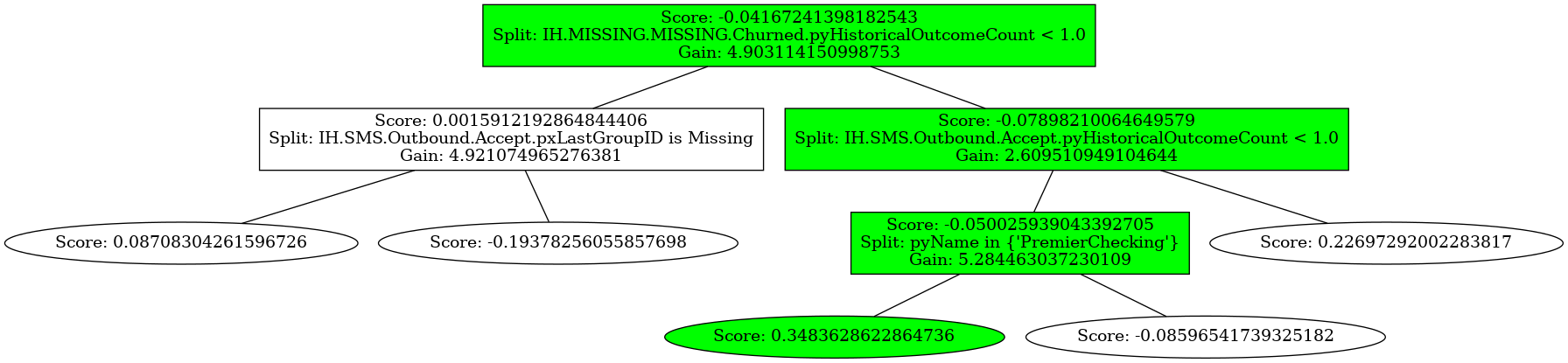
Plot prediction path

With this tree, of course we can also show how a tree would score a set of input data ‘x’. Simply pass a dictionary with variable:value pairs to plotTree’s “highlighted” parameter, and that path is highlighted:

Trees.plot_tree(18, highlighted = {"IH.MISSING.MISSING.Churned.pyHistoricalOutcomeCount":2, "IH.SMS.Outbound.Accept.pyHistoricalOutcomeCount":0, "pyName": 'PremierChecking'});

Of course that also works if we define x first and then feed that as the highlighted parameter.

x = {"IH.MISSING.MISSING.Churned.pyHistoricalOutcomeCount":2, "IH.SMS.Outbound.Accept.pyHistoricalOutcomeCount":0, "pyName": 'NotPremierChecking'}
Trees.plot_tree(18, highlighted=x);

Thus far we’ve only look at tree 18, but of course we can plot different trees as well. This is also where these visualisations aren’t always as useful, because the trees can get quite large and hard to read:

Trees.plot_tree(30);

Note it is possible to export these trees by calling functions on the raw model, such as ‘write_png’ or ‘write_pdf’:

Trees.plotTree(4, highlighted=x).write_png('Tree.png')
Trees.plotTree(4, highlighted=x).write_pdf('Tree.pdf')

Random input data

For this demo, I want to generate some random input parameters, so a quick function to do that is this:

def sampleX(trees):
    from random import sample

    x = {}
    for variable, values in trees.all_values_per_split.items():
        if len(values) == 1:
            if "true" in values or "false" in values:
                values = {"true", "false"}
            if isinstance(list(values)[0], str):
                try:
                    float(list(values)[0])
                except:
                    values = values.union({"Other"})
        x[variable] = sample(list(values), 1)[0]
    return x


randomX = sampleX(Trees)

Replicating scores

Lastly, with a given x and each scoring tree both stored, we can replicate the score the models would give to that customer by simply letting each tree predict a score. By calling ‘getAllVisitedNodes’, we get an overview of all visited nodes, each split that was performed and the scores contributed by each individual tree. By default this is sorted by their scores. This also gives us an idea of the relative ‘importance’ of each tree for the final prediction.

scores = Trees.get_all_visited_nodes(randomX)
scores

shape: (50, 4)

treeID	visited_nodes	score	splits
i64	list[i64]	f64	str
0	[1, 2, … 7]	-0.598675	"[{'pyName in { AutoUsed48Month…
1	[1, 21, 23]	-0.464293	"[{'pyGroup in { DepositAccount…
2	[1, 2, … 15]	-0.402499	"[{'pyName in { AutoUsed48Month…
3	[1, 11, … 23]	-0.355028	"[{'pyName in { PremierChecking…
4	[1, 2, … 32]	-0.23541	"[{'pyName in { AutoUsed48Month…
…	…	…	…
45	[1, 2, … 13]	-0.016589	"[{'pyName in { AutoUsed48Month…
46	[1, 2]	-0.069158	"[{'IH.SMS.Outbound.NoResponse.…
47	[1, 11, … 19]	0.220699	"[{'pyName in { AutoUsed48Month…
48	[1, 23, … 32]	-0.184534	"[{'pyName in { AutoUsed48Month…
49	[1, 2, … 6]	0.080806	"[{'Customer.NetWealth < 18233.…

Now, to get to the final score we simply sum up the scores, and then normalize them to a range between 0 and 1:

import math

1 / (1 + math.exp(-scores["score"].sum()))

0.0036005213905183553

And to simplify this even further, simply call the ‘score’ function to get the final score.

Trees.score(randomX)

0.0036005213905183553

Finally, we can also plot the contribution of each tree towards the final propensity of the prediction. Simply call the plotContributionPerTree function with a given x. This shows, for each individual tree, the scores, the cumulative mean of those scores and the running propensity. Here you can clearly see that the average score is quite negative, so as we would expect the final propensity is also quite low.

Trees.plot_contribution_per_tree(randomX);

These are the current features of the ADMTrees class. As always, if you have suggestions, please do not hesitate to open a GitHub issue or pull request!